1. GAMS introduction
GAMS, short for General Algebraic Modelling System, is a commercial optimization software developed and sold by GAMS Development Corporation. Its speciality is describing and solving large-scale optimization problems with millions of variables and equations. It comprises a special purpose model description language based on sets, parameters, variables and equations. It supports solving linear, mixed integer, quadratic and nonlinear optimization problems.
Sets and parameters are input data that describe the system to be optimized. Equations describe the system structure. Variables values of an optimal solution are model output.
1.1. Example (1) – Fuel station
The following code section is a complete model of a hypothetic fuel station for electric vehicles that generates its electricity from renewable sources and has an electric storage. Highlighted are non-functional inline comments that provide explanations and data sections.
Sets (input) in this model are electricity generation technologies i (photovoltaics, wind onshore and offshore) and timesteps t (1…8760). Each renewable source has a normalised timeseries parameter cf(t,i) that is defined over the whole year with time resolution of one hour. Electric cars are modelled as a demand timeseries d(t). For brevity, all timeseries are generated from random numbers. Both storage and electricity generation have attached investment costs cs in k€ per MWh storage capacity and c(i) in k€ per MW generation capacity.
Optimization variables (model output) in this model are the generation capacities per technology x(i) in MW and the storage size s in MWh. The variable to be minimized is z, the total cost for satisfying the demand d(t) in each timestep over the whole year. Variable st(t) simulates the storage filling level in each timestep. All energy quantities are limited to positive values by a single positive statement.
The main equation cost sets the value for variable z. It is the cost function, whose value z is to be minimized. Equation pp(t) calculates the value for helper variable tp(t), the total energy production per timestep. Equation dd(t) assures demand satisfaction either from production or storage and is the main optimization constraint in this model. Equation storage(t) calculates the filling levels for each timestep. Variable sell(t) enables the model to throw away excess energy. Equation ss(t) limits filling level to the storage capacity. The final equations ss0(tfirst) and ssN(tlast) set boundary conditions for the storage filling level.
$title Electric fuel station model (fuelstation.gms)

Sets
    t          time               / 1*8760 /
    i          type of production / pv, windon, windoff /
    tfirst(t)  first timestep
    tlast(t)   last timestep;

    tfirst(t) = yes$(ord(t) eq 1);
    tlast(t)  = yes$(ord(t) eq card(t));

Parameters
    cs      cost of storage tank (k€ per MWh) / 100 /
    c(i)    cost of plant (k€ per MW) / pv 3000, windon 1500, windoff 2500 /
    d(t)    demand (MWh)
    cf(t,i) relative (normalized to 1) production of plants;

    d(t) = uniform(0,1);
    cf(t,'pv') = min(max(0,power(sin(ord(t)/24*3.14/2),4)+normal(.1,.1)),1);
    cf(t,'windon') = min(max(0,uniform(0,1)),1);
    cf(t,'windoff')= min(max(0,sqrt(sqrt(uniform(0,1)))),1);

Variables
    x(i)       size of production facilities (MW)
    s          size of accumulator (MWh)
    st(t)      evolution of accumulator SOC (MWh)
    tp(t)      total production of plants per timestep (MWh)
    z          total cost (k€)
    sell(t);

Positive Variables x, s, st, sell;

Equations
    cost       total cost equation
    pp(t)      calculates tp (total production) from cf and x
    dd(t)      assures that demand is always satisfied
    storage(t) new_storage = storage + input - demand
    ss(t)      simulates the capacity of the accumulator
    ss0(t)     initial storage content
    ssN(t)     final storage content;

    cost..         z          =e= sum(i, x(i)*c(i)) + cs*s;
    pp(t)..        tp(t)      =e= sum(i, cf(t,i)*x(i));
    dd(t)..        d(t)       =l= tp(t) + st(t);
    storage(t)..   st(t+1)    =e= st(t) + tp(t) - d(t) - sell(t);
    ss(t)..        st(t)      =l= s;
    ss0(tfirst)..  st(tfirst) =g= s/2;
    ssN(tlast)..   st(tlast)  =g= s/2;

Model  fuelstation / all / ;
Solve  fuelstation using lp minimizing z ;
Display  x.l, s.l;
1.2. Sets
Sets are collections of items. Each item is identified by its string representation, a string which can be up to 63 characters long and must start with an alphabetic or numeric character. In unquoted strings, the only allowed characters are alphabetic and numeric characters, plus (+), minus (-) and the underscore (_). In quoted strings spaces and special characters are allowed. Set elements are separated by commas or line breaks. Example:
set supply sites / Seattle, Chicago, "New York", Washington /;
Numeric items in general have no special meaning or semantics. There is, however, syntactic sugar to automate creating sets with numeric elements. The following example creates a set with 168 consecutive integer elements 1 to 168:
set t timesteps / 1*168 /;
Subsets can be created by naming the superset in parenthesis after the set name. Elements of the subsets then need to be elements of the superset. Subsets used for special rules that only apply to a subgroup of modelled things.
set bigsupply(supply) special sites / Seattle, Washington /;
Elements for sets can not only be explicitly named, but also computed. This happens usually for subsets of a static superset. The syntax is subset(superset) = yes$condition. The command includes those items of the superset in the subset that fulfil the condition. Conditions are comparison expressions that can include sets, parameters and functions (described in section 1.6). The following example creates the subset tlast by only including the last element of t by using the set functions ord and card that exploit implicit ordering of static sets like t (called ordered set):
set t timesteps / 1*8760 /;
set tfirst(t) initial timestep;
tlast(t) = yes$(ord(t) eq card(t));
Multi-dimensional sets can be defined like subsets, but with multiple supersets. Elements are defined by a concatenation of set elements with the dot (.) character:
set co commodities / Coal, Gas, Oil /;
set pro process names / gt, pp, cc /;
set process_chain(co,pro) / Coal.pp, Coal.cc, Gas.gt, Oil.pp /;
It is possible to assign an alias to any set. This can be useful either for having a shorter name and is necessary for defining certain types of equations.
alias(knownset,alias1,alias2,…);
alias(node,i,j);
1.3. Parameters
Parameters are n-dimensional matrices of numerical values, defined over one or several sets, the so-called onsets. Scalar parameters without onsets are possible, too. Like with sets, an explanatory text can be added between parameter name (loss) and data section (/…/):
parameter loss energy losses per km / 0.001 /;
Here is a typical example for a one-dimensional parameter:
set tech / pv, windon, windoff, hydro /;
parameter invcost(tech) investment cost per kW
         / pv 2000, windoff 1500, windon 1100, hydro 900 /;
A more advanced example for a two-dimensional parameter that mixes explicit values and computed values to create a symmetric distance matrix among a set of nodes. Unmentioned set element pairs automatically have the value zero:
set node / a, b, c, d /;
parameter dist(node, node) / a.b 5, b.c 7, c.d 5 /;
alias(node,i,j);
dist(j,i)$(dist(i,j)) = dist(i,j);
There is another format for entering data for dense, high-dimensional data: the table command. Usually, the nth dimension is used as captions for columns, while the remaining (n-1) dimensions are used as row captions. The following example shows a typical three-dimensional parameter definition:
set site / AT, CH, DE /;
set commodity / Gas, Wind /;
set attribute / invcost, instcap /;
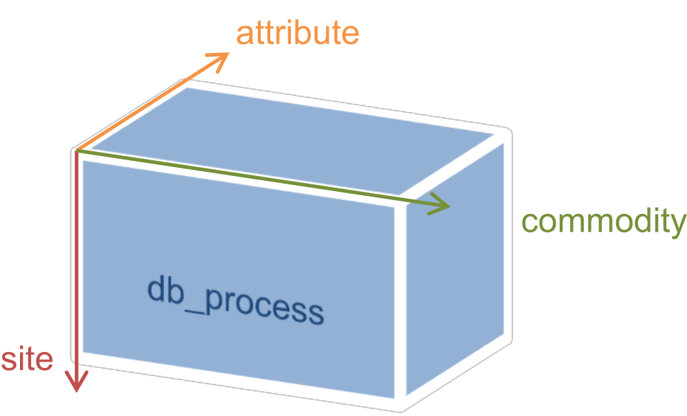
table db_process(site,commodity,attribute)
invcost instcap
AT.Gas 800 470
AT.Wind 1600 2400
CH.Gas 750 650
CH.Wind 1900 5500
DE.Gas 850 35000
DE.Wind 1400 23000;
The resulting data structure can be visualised as a cube/array with three dimensions. Each direction corresponds to one of the onsets:
1.4. Variables
Variables are declared like parameters, except that their value is not pre-defined. It is the solver’s task to find values for all variables that minimize or maximize the objective function. Equations can limit the allowed value range or even force some variables to a fixed value.
variable z total cost;
variable p(tech) output power (kW) per plant;
variable x(tech) building decision per plant;
By default, variables are unconstrained real values. Additional statements allow restricting the allowed range to positive, binary or integer values:
positive variable p;
binary variable x;
After a successful optimization run, the following attributes of each variable are set:
| Attribute | Explanation |
|---|---|
| .l | Activity level. Value of variable in optimal solution. |
| .m | Marginal. Change in cost function value if x is changed by one unit. |
1.5. Equations
Equations are the core of every GAMS model. They describe the connections between parameters and variables. Sets provide means to restrict equations to certain groups of elements. It is beyond the scope of this document to explain their syntax. GAMS provides more than enough examples and documentation. Section 1.7 lists the most important documents.
1.6. Auxiliary statements
Apart from the aforementioned elements, there are a number of other language features that allow for easier data handling, debugging and result display. The following table summarises frequently used statements.
| Command | Explanation |
|---|---|
| display | Displays contents of sets, parameters or variables after successful solve. |
| solve | Solves a problem created by the command model. |
| model | Creates a problem from a set of equations. all uses to all equations. |
For example, to display the optimal value of decision variable x after simulation, the command display x.l; can be used.
1.7. Further reading
A good introductory document with all common language features is the GAMS Users Guide:
C:\GAMS\win64\xx.y\docs\userguides\GAMSUsersGuide.pdf
A more in-depth language reference is the extended McCarl GAMS User Guide:
C:\GAMS\win64\xx.y\docs\userguides\mccarl\mccarlgamsuserguide.pdf
A third source of inspiration is the GAMS Model Library that can be found in the GAMS main menu.